Computing time series volatility

Computing stock price volatility with Data-Forge

This blog post was exported from Data-Forge Notebook. You can edit and evaluate this notebook with Data-Forge Notebook.

This is an example JavaScript notebook that shows how to use the percentRange function from the Data-Forge code library to compute percent volatility for time series data.

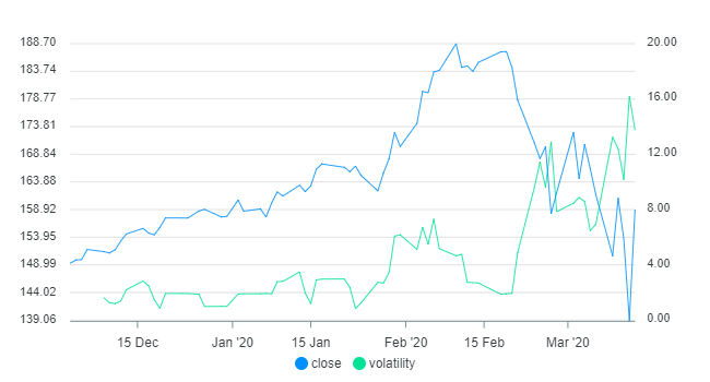
In this post we are computing the 5-day volatility for Microsoft's stock price. This is particularly interesting because we can see how the recent plunge in the stock market has affected volatility of the stock.

Install code libraries

If you are using Data-Forge Notebook simply requiring the libraries (as shown in the next section) means those libraries will be automatically installed. If you are using Node.js you'll have to install the code libraries manually as follows:

npm install --save datakit data-forge dayjs

Import code libraries

Import the code libraries we need for this example:

const datakit = require("datakit");
const { DataFrame } = require("data-forge");
const dayjs = require("dayjs");

Load data

Load the data from a CSV file into a dataframe and preview the first 3 rows:

const data = 
    await datakit.readCsv("./MSFT.csv", { // Load data.
        parser: { 
            timestamp: 
                v => dayjs(v, "YYYY-MM-DD").toDate(), // Parse dates.
        },
    }); 
let df = new DataFrame(data);   // Load data into dataframe.
display(df.head(3));            // Preview our data.

index	timestamp	open	high	low	close	volume	SMA
0	2019-12-03 00:00:00	147.49	149.43	146.65	149.31	25192145	146.33500000000004
1	2019-12-04 00:00:00	150.14	150.1799	149.2	149.85	17580617	146.78433333333336
2	2019-12-05 00:00:00	150.05	150.32	149.48	149.93	17880601	147.20733333333337

Compute volatility

Here we compute percentage volatility of the closing price over a 5-day period (how much % the stock has changed over the week):

const volatility =
    df.getSeries("close")       // Get the "close" series from the dataframe.
        .percentRange(5)        // Compute % volatility with a 5-day period.
        .round(2);              // Round to two decimal places.
display(volatility.head(3));    // Preview computed volatility.

index	value
4	1.61
5	1.26
6	1.2

Integrate volatility

Integrate the computed % volatility back into the dataframe:

df = df.withSeries({ volatility }); // Integrate "volatility" column.
display(df.skip(4).head(3));        // Preview integrated data.

index	timestamp	open	high	low	close	volume	SMA	volatility
4	2019-12-09 00:00:00	151.07	152.21	150.91	151.36	16741350	147.95533333333333	1.61
5	2019-12-10 00:00:00	151.29	151.89	150.765	151.13	16481060	148.18666666666667	1.26
6	2019-12-11 00:00:00	151.54	151.87	150.33	151.7	18860001	148.48233333333334	1.2

Plot chart

Plot the closing price against our computed % volatility. Notice how volatility increases quickly as the stock prices drops:

display.plot(
    df.toArray(), 
    {}, 
    { x: "timestamp", y: "close", y2: "volatility" } 
);

Chart

What can we do with this?

Volatility is used to assess how much a time series is fluctuating. You can use this in your trading strategy however you like. Does your strategy rely on highly volatile stocks? This is how you can measure that. Do you prefer to invest in less volatile stocks? This can do that as well.

Volatility is also a useful measure of potential risk and/or profit. The amount of movement in the past day, week or month gives you some indication of how far down (potential risk) or far up (potential profit) the stock might move if you held a position for that long. Better yet use a moving average of volatility to take the average of past volatility into account.

You might even use volatility as a market filter, only trading either if the market is highly volatile or less volatile, depending on the needs your strategy!

You can edit and evaluate this example notebook with Data-Forge Notebook

Menu